After building a WebScraper with BeautifulSoup, I decided to visualize the data with Plotly. Note: for the book data “prices and ratings here were randomly assigned and have no real meaning” as stated by the source website books.toscrape.com because the website it used for testing purposes.

Unfortunately the official documentation is not super helpful and hasn’t been updated in a while, you can tell this because it talks about embedding graphs on tumblr. There is a WordPress plugin for plotly but it hasn’t been updated in 7 years so it doesn’t work with modern WP.

Third parties are more helpful. You can embed charts in WordPress using chart studio iframes and the WordPress custom iframes require a buisness or ecommerce plan, otherwise the code won’t save. Using the HTML tab of chart studio share feature results in a static graph that does save. Like so:

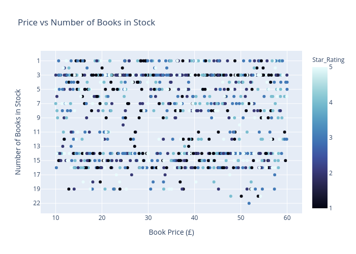
The code to create this graph is pretty simple. Renamed the x and y axes and added an appropriate title. I also included a third variable: star_rating which is discrete and a 1-5 stars as the color for the scatterplot.
For the star ratings, I debated whether or not it is appropriate to use a color gradient from 1-5 or discrete (unordered), and I settled on the former.

import plotly.express as px
fig = px.scatter(df, x='Price£', y='Stock_Status_Num',color='Star_Rating',   color_continuous_scale='ice', labels = {
        "Price£": "Book Price (£)",
        "Stock_Status_Num": "Number of Books in Stock"},
        title ='Price vs Number of Books in Stock')
fig.show()

py.iplot(fig, filename='price-stock-books', auto_open=True)

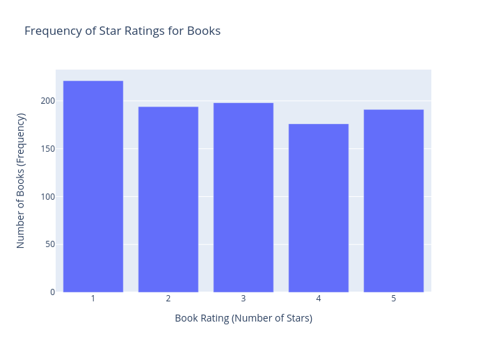
I can’t see any clear trends. So for the next graph I wanted to see if the how many books there are by star rating

Using pandas, I first grouped by the number of stars and counted the frequency, then added an appropriate title and axes etc:

dfg = df.groupby(["Star_Rating"]).count()
fig = px.bar(dfg, x=dfg.index, y="URL", labels = {
        "Star_Rating": "Book Rating (Number of Stars)",
        "URL": "Number of Books (Frequency)"}, title="Frequency of Star Ratings for Books")
fig.show()
py.iplot(fig, filename='star_freq-books', auto_open=True)

Conclusion

Lots of cool stuff to explore with plotly, especially with creating interactive graphs and dashboards. With more complicated data I could make more interesting and insightful graphs.

In this article, I walk you through the building a program takes online book data on books.toscrape.com and stores it in a local SQLite database. You can see all the code for the completed project here.

Introduction

Data exists somewhere, but we want it somewhere else. This is the fundamental problem posed in data engineering; it’s a problem that occurs again and again when dealing with data. In some cases (like ours) that data currently exists on a website and we want to organize it in a tabular way and store it locally (or on the cloud) so that it can easily be retrieved later.

Websites are made of code. When you visit a webpage, you’re requesting access to that code. Our browsers translate this code into interactive visual experiences most of us understand to be websites. If you want to really see what is going on behind the curtain all you need to do is right-click somewhere on a web page and click “Inspect” or “View page source” and you will instantly be greeted by nested trees of information containing text, links, images, and tables.

For this project, I used books.toscrape.com as the data source. This website is designed to be scraped which makes it the perfect place to practice.

Implementation

One way to get a page’s source code in python is to use the requests library.

import requests

page_url = "http://books.toscrape.com/catalogue/a-light-in-the-attic_1000/index.html"
page = requests.get(base_page_url)

We want to check if the website actually received our request. If the website admins prevent our IP address from accessing content or if we mistype the url we’re trying to access we will receive a different status code. You can read more about status codes here.

if page.status_code == 200: #200 means everything went okay!
    pass
else:
    raise Exception("Invalid Status Response Code")

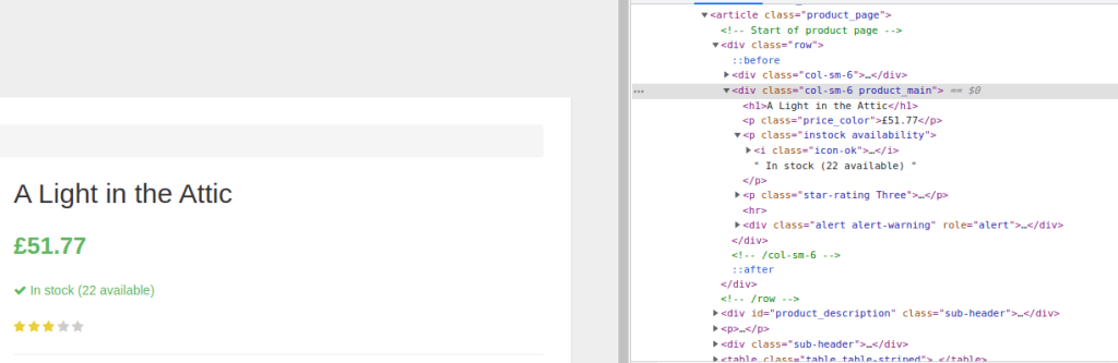
Unfortunately requests leaves us with an unwieldy mess. Having the source code for an entire web page is not extremely helpful by itself. Thankfully, we can use a different library called BeautifulSoup to parse (or sift) through all the HTML and extract the useful nuggets of information we want.

soup = BeautifulSoup(page.text, 'html.parser')

Now that we have our “soup” we can search for specific tags and then iterate over them. It sometimes takes a little extra wrangling with common functions like replace (replaces certain characters with other characters) and strip (removes white space from either side).

for book_tree in soup.find_all(class_='col-sm-6 product_main'):
    title = book_tree.find("h1").contents[0]
    price = book_tree.find(class_="price_color").contents[0]
    price = price.replace("Â", "")
    stock_status = book_tree.find(class_="instock availability")
    stock_status = stock_status.contents[2].replace("\n", "")
    stock_status = stock_status.lstrip().rstrip()

Once we have this data we want to first store it in a dictionary (in memory) for clarity, flexibility, and ease of use. We include all the relevant info we want to store, like the url page or when we scraped the page (web pages are sometimes updated!).

import datetime

return {"url": url,
        "title": title,
        "price": monetary(price), #monetary turns str to float
        "stock_status": stock_status,
        "date_scraped": datetime.now().strftime("%m/%d/%y")
        }

Finally we want to store that dictionary in a more permanent place. One option is to use pandas and store the data directly in a csv (comma seperated values). However the csv format is not native to data storage and can cause issues when trying to read and write at the same time, or when trying to insert.

Common industrial databases like MySQL or PostgreSQL are designed to handle online requests from multiple users simultaneously, so setting them up is a chore and should only be done if you actually need that functionality.

My choice is to use SQLite, a lightweight local relational database that’s included with python. We first need to make a table, and if the table already exists make sure our code can handle that scenario.

conn = sqlite3.connect(db_path)

# cursor object
cur = conn.cursor()

# Creating table
table = """
        CREATE TABLE Books (
        URL TEXT NOT NULL,
        Title TEXT NOT NULL,
        Price£ FLOAT NOT NULL,
        Stock_Status TEXT NOT NULL,
        Date_Scraped TEXT NOT NULL
        );
        """

try:
# if the table does not exist yet, below line with throw error
    cur.execute(table)
    if verbose==True: 
        print("Table created.")
except sqlite3.OperationalError as e:
    #if the table already exists
    if verbose==True:
        print(e)

    # Close the database connection
    conn.close()

More complicated databases should have primary and foreign keys to reduce redundancy, but here the data is so simple there’s no reason to implement a more complicated structure.

Now that we have a database and a table, we can insert data into it like so:

conn = sqlite3.connect(db_path)
sql = ''' 
      INSERT INTO Books(URL,Title,
              Price£,Stock_Status, Date_Scraped)
              VALUES(?,?,?,?,?) 
      '''
cur = conn.cursor()
data_tuple = (input_dict["url"], 
              input_dict["title"],
              input_dict["price"], 
              input_dict["stock_status"],  
              input_dict["date_scraped"])                               
cur.execute(sql, data_tuple)
conn.commit()
  
    
# Close the database connection
conn.close(

If you can do one book….you can scrape a whole lot. Using a similar methodology to single book information: you grab links to all the books on the browsing page.

base_page_url= "http://books.toscrape.com/catalogue/page-"+str(page)+".html"

url_list = []
page = requests.get(base_page_url)

soup = BeautifulSoup(page.text, 'html.parser')
   for book_tree in soup.find_all(class_='image_container'):
       for link in book_tree.find_all('a'):
           url = "http://books.toscrape.com/catalogue/" + str(link.get('href'))
           url_list.append(url)

And all that’s left is to go through each url and scrape that particular book! It’s a pretty simple implementation using a for-loop. One more detail though is to add a pause between requests. We don’t want to spam a website with requests and look like a denial of service attack.

 for url in url_list:
     add_book_to_database(db_path=db_path,       input_dict=scrape_single_book_page(url)) #scrape each url
     time.sleep(seconds_to_wait_between_scrapes) #wait a little

Done!

Conclusion

Now that wasn’t too hard, was it? Data scraping is an essential tool in any data scientist or engineer’s arsinel. Note that I didn’t include any code to prevent duplicate entry rows. For example, if you only wanted to scrape a website once a day you could check no row already exists today at that url. However, for a real world example there might be reasons to want to scrape the same data multiple times per day which is why I’m leaving it as-is.

You can find the full repo here. Thanks for reading!

Introduction

Are you a typical UFC viewer? Have you ever wondered if the ranking next to a UFC fighter’s last name actually means anything? I was curious and wanted to answer this question by investigating the data.

Why The Rankings Matter

There are real implications for the fighters: their UFC ranking is an important part of a UFC Fighter’s brand. Many UFC fighters use these rankings to decide who they should accept fights against in addition to impacting their image in an entertainment industry where being seen as better means a better paycheck. Their UFC ranking is an important part of a UFC Fighter’s brand. One ranked UFC fighter went as far as to say: “the ranking system, they put us in a position — how come the guy #5 or #6 is fighting a guy that’s not even in the rankings? Because of the ranking system, it’s kind of like a limit which I don’t agree with … because of that, I don’t want to take a fight against someone not in the rankings“.

The Data

The best way to decide if the rankings matter is by using statistics to analyze what the rankings are before each fight happens. BUT to my surprise, this information isn’t stored anywhere I could find online (if it was, it would’ve saved me a bunch of time). So I went out and re-watched all of the events of the last few years and tracked what the rankings were at the time of each fight that included at least one ranked fighter. I collected the data in a google sheet file (which is analogous to an Excel or csv file).

There are way more potential match-ups (15 vs 14, 8 vs 5, 8 vs 7 etc) than the number of data points that exist in my sample (around 200 fights that include two ranked fighters). For my analysis I used the difference between rankings as a continuous variable which assumes the difference in skill between rank 1 and rank 2 is the same as between rank 14 and rank 15. It is reasonable to expect the larger the difference in ranking the more likely it is the higher ranked fighter wins, and this is one barometer I will use to evaluate the rankings.

A quick primer on Bayesian statistics and logistic regression

The basic idea behind Bayesian statistics is that probability is about degrees (or magnitudes) of belief. For example: If I am completely certain of an outcome, it has a 100% chance of happening. This contrasts with the frequentist (traditional view) that probabilities are the long-run frequency of an event occurring.

The beauty of Bayesian statistics is that instead of creating a single parameter estimate, it produces a frequency distribution of all the possible parameter values and specifies how confident we should be in each parameter.

So what is logistic regression?

Logistic regression is based on linear regression (which fits a line through data in a way that minimizes the sum of their squared errors). Logistic regression uses a logit squashing function to turn the outputs of a linear regression into a range between 0 and 1. Whereas linear regression could be used to predict a continuous variable—for example height in inches or the price of a stock, logistic regression tackles classification problems—like whether or not a fighter will win a UFC fight, or if a picture is of a cat or dog.

Analysis of the data

In this specific example, a frequentist logistic regression model only produces singular intercept and coefficient estimates, by using a Bayesian model I’m able to estimate a distribution of possible intercepts and a distribution of coefficient estimates.

The model specification not including the logit transform is simple:

y = Intercept + Rank_Difference * x

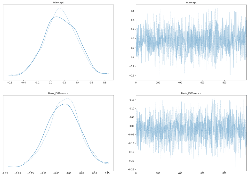
After applying the markov chain monte carlo (MCMC) sampling to some reasonable priors and hitting the “inference button”, my program spit out posterior distribution estimates for what our model parameter coefficients should be:

The shocking thing about this, is that the mean of the rank_difference coefficent is actually negative (!!!) that means that a fighter ranked 9 fighting a fighter ranked 10 has a higher probability of winning than a fighter ranked 5 facing a fighter ranked 10.

You should take this with a large grain of salt though, my posterior estimates indicate a lot of uncertainty and a positive coefficient is also believably consistent with the data.

In terms of model specification, the trace plots and pair plot seem normal:

Conclusions

There is an important discussion to be had about the role of rankings in sports. In sports leagues like the NBA or NFL rankings are mainly determined by record (with some tie-breaking rules) and conference. Only in the playoffs are these rankings shown, and they are usually very reliable indicators of which team is better. For example, in the NBA 80% of teams who win the championship are seeded first or second out of 8 (this means being top 4 since there are two conferences).

But in leagues where the data is incredibly sparse (there are many more UFC fighters and College Football teams than the 30 NBA teams or 32 NFL teams) and the rankings are voted on (not automatically determined by a formula) it is vital to hold the rankings accountable because they simply the opinions of people: “[UFC] Rankings were generated by a voting panel made up of media members. The media members were asked to vote for who they feel are the top fighters in the UFC by weight-class”. The higher ranked fighter only wins 53% of the time. You will get way better results by looking at vegas odds for determining who the best fighters in the world are.

Further work could collect more data and add additional variables of interest.

Thanks for reading!

You can find my google colab notebook here